Homework 2

Due 5/3/06

1. Consider an ideal ring polymer, that is one with no interactions, topological or otherwise. It is composed of N beads with positions $({\bf r}_1,\dots,{\bf r}_N)$. Consider $\langle \vert{\bf r}_{N/2} - {\bf r}_1\vert^2\rangle$. Consider the same quantity when the bond between beads $1$ and $N$ are cut giving a linear chain. Calculate the ratio of these two quantities.

2. Consider an infinitely long ideal polymer chain in three dimensions with a step length $l$. If a monomer is at position ${\bf r}_0$, calculate the probability density that another monomer with be at position ${\bf r}$. Assume that $r >> l$, that is don't worry about short distance effects of order the chain step length. You can get the form of the result in any dimension but don't have to. Hint: The answer is the sum of probabilities for different arclengths. This sum can be approximated by an integral. The integral can be done by Fourier transformation with respect to ${\bf r}$. It can also done by a change of variables if you're working in three dimensions.

3. Multifractals Multifractals appear in a large variety of systems: turbulence, chaotic dynamical systems, nonequilibrium aggregation models, and are thought to even appear in financial markets. In this problem we'll start exploring these fascinating systems. The following model was first introduced in understanding turbulence, see R. Benzi, G. Paladin, G. Parisi and A. Vulpiani J. Phys. A: Math. Gen. 17 (1984) 3521-3531.

Consider the field $\phi({\bf r})$, is this case it could be the energy dissipation as a function of position for a turbulent fluid. Turbulence is believed to be self similar so we model the physics to be the same at all length scales down to a cutoff length $a$. We think of large scale eddies breaking up into smaller scale ones, and those in turn breaking up. Although the model here seems very crude in many ways, it captures essential features of the physics that are inaccessible by many other involved mathematical calculations.

The model is depicted below.

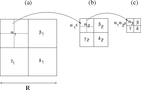
We start off in (a) by breaking up the field into four parts (eddies) so that the proportion of the total dissipated power per unit volume (power density) in the four sub-boxes are $\alpha_1$, $\beta_1$, $\gamma_1$, and $\delta_1$ (which are all positive and add up to unity). We assume these numbers are randomly drawn from some probability distribution, so that the probability distribution for $\alpha_1$ is $P(\alpha_1)$. Many choices can be made for this distribution and will effect the physics that follows. Now we assume that system breaks itself up further in a manner similar to what it just did but now at a smaller scale. So in (b), the upper left hand box then divides its dissipated power in the same way among four boxes. $\alpha_2$, $\beta_2$, $\gamma_2$, and $\delta_2$ are drawn randomly in the same way as before. However the power density for this sub-box is scaled by an overall factor of $\alpha_1$. Therefore the total power in the upper left hand box of (b) at this new level is $\alpha_1 \alpha_2$. We can continue to subdivide this way. The final box, (c), shows the eddies breaking up at a further level. Now the total power density in the upper left hand box in (c) is $\alpha_1\alpha_2\alpha_3$.

This process continues all the way down to a cutoff length $a$. If there are $N$ generations of subdivision, The ratio of the initial box length $R$ in (a) to $a$ is $2^N$. That is

$$R/a = 2^N.$$ (1)

Call the complete field for all space constructed using the above procedure $\phi({\bf r})$. Its values depend on the realizations of the random variables (e.g. $\alpha_i$) used to construct it. We would like to know various averages of $\phi$ averaged over all realizations of these random variables.

a

Calculate $\langle \phi^m \rangle$. Take $m$ to be any positive exponent. Express your answer as a function of the number of generations $N$, and in terms of moments of the distribution $P(\alpha)$ mentioned above, that is $\langle \alpha^m \rangle$.

b

Using eq. 1, write $\langle \phi^m \rangle$ as a function of $R$, the size of the system. Your answer should still depend on the moments of the same distribution as in (a).

c

Calculate the moments $\langle \phi^m \rangle$ explicitly in the case where the $\alpha$'s can only take on two distinct values both with equal probabilities. Note that $\langle \alpha \rangle = 1$ because the total power injected at a larger scale is accounted for by the power present at smaller scales. So this model has one free parameter characterizing the width of $P(\alpha)$.

4. Verify your results for problem 2 numerically. The statistics can be improved by binning over spherical shells, but it is not necessary for you to do this.

a

Write a function to generate a random walk of $N$ steps.

b

Keep track of the number of times it hits a site on the lattice by including a density map in the form of a three dimensional array, or a one dimensional array if you're binning over spherical shells.

c

By calling the random walk function repeatedly, the density map becomes smoother.

d

By looking along the x direction, after sufficiently many runs, you can compare your answer to the analytical result. Alternatively if you're binning over spherical shells you can get the answer by examining the one dimensional array.