Next: About this document ...
Up: magnetic_field
Previous: Three dimensions and the
In this appendix we derive the expression for Landau diamagnetism of free
electrons. Our approach will be to derive the result first for 2- from which
we will easily be able to obtain the 3- result by integrating over
from which
we will easily be able to obtain the 3- result by integrating over  .
.
Firstly, we remind ourselves of some statistical mechanics. It is convenient to
calculate the grand partition function,  where
where
![\begin{displaymath}
{\cal Z} = {\rm Tr} \exp[\beta(\mu N - {\cal H})] ,
\end{displaymath}](img140.png) |
(49) |
where  is the number of particles and
  is the Hamiltonian.
The trace
is over all states for a given and over all . This ensemble, where both
and
is the Hamiltonian.
The trace
is over all states for a given and over all . This ensemble, where both
and  are allowed to vary, is called the ``grand canonical ensemble''.
is related to the ``grand potential'',
are allowed to vary, is called the ``grand canonical ensemble''.
is related to the ``grand potential'',  , by
, by
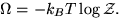 |
(50) |
The mean number of particles is given by
 |
(51) |
which implicitly determines  . is related to the free energy
 by
by
 |
(52) |
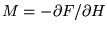
Note that is considered as a function of and so differentiating
the right hand side of Eq. (A4) with respect to (keeping
constant) gives
 |
(53) |
This will be useful later. Note that a lot of confusion in statistical
mechanics
comes from a lack of understanding of what is being kept constant in partial
derivatives. Once the correct value of has been determined for a given
, we determine the magnetization from
 |
(54) |
where  is the magnetic field and the derivative is at fixed .
Note that in general
we need to determine
is the magnetic field and the derivative is at fixed .
Note that in general
we need to determine  from
from
 rather
than
rather
than
 , because the number of
particles is kept constant when the field is applied, not the chemical
potential. However, as we shall see, they both give the same result to lowest
order in , the case of interest here, because of Eq. (A5).
The susceptibility is then found from
, because the number of
particles is kept constant when the field is applied, not the chemical
potential. However, as we shall see, they both give the same result to lowest
order in , the case of interest here, because of Eq. (A5).
The susceptibility is then found from
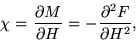 |
(55) |
so we have to compute the  term in the free energy.
A useful feature of the grand canonical ensemble is that, for
non-interacting particles, the grand potential factorizes into a product of
grand potentials for each single particle state, and so the grand potential is
a sum of grand potentials for single particle states. Hence, for free
electrons,
![\begin{displaymath}
\Omega = -k_B T \sum_k 2 \ln[ 1 + e^{\beta(\mu - \epsilon_k)} ] ,
\end{displaymath}](img154.png) |
(56) |
which can be conveniently be expressed in terms of the density of states,
 (for both spin species) by
![\begin{displaymath}
\Omega = -k_B T \int_0^\infty g(\epsilon)
\ln[ 1 + e^{\beta(\mu - \epsilon_k)} ] \, d\epsilon .
\end{displaymath}](img156.png) |
(57) |
Consider first  . We are interested in the low-
 limit where, as
discussed in class, the difference between and its
limit where, as
discussed in class, the difference between and its  limit,
 , is negligible.
As discussed above is a constant
, is negligible.
As discussed above is a constant
 .
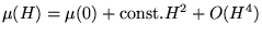
and so, for small and
.
and so, for small and
where the last equality is from Eq. (14).
For  , where
  is negligible, is just
  with
with
 , and so
 |
(61) |
in agreement with Eq. (15), which gives the energy per electron rather
than the total energy as here.
Now we add a field, which changes in two ways.
Firstly it changes the density
of states, as we have discussed in detail in the main part of the text.
Secondly it changes the chemical potential, so
 . However, we shall see that the change in due to the
change in with does not affect the free energy
. However, we shall see that the change in due to the
change in with does not affect the free energy  , so we just
focus here on the change in
due to the modification of the density of states.
, so we just
focus here on the change in
due to the modification of the density of states.
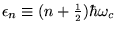
In the presence of a field ,
the energy levels take the discrete values
 and so
![\begin{displaymath}
\Omega(H) = -k_B T {A m \over \pi \hbar^2} \hbar \omega_c
\sum_n \ln[ 1 + e^{\beta(\mu - \epsilon_n)} ] ,
\end{displaymath}](img172.png) |
(62) |
which is to be contrasted with Eq. (A10) for .
The difference
is that Eq. (A14) can be though of as a discretized approximation to
Eq. (A10) of the sort that is often used in numerical analysis.
The integral over a range of width
 is replaced by
times the value of the the integrand at the
midpoint of the interval.
The difference between the integral and the approximation to it using this
``midpoint rule''
is well known (see e.g. Numerical Recipes in C (or in Fortran) by
Press et al, Eq. (4.4.1)), and can be easily derived by replacing the function
in each interval by a polynomial, doing the integral with the first few terms
of the polynomial, and summing over intervals. The result can be expressed as
is replaced by
times the value of the the integrand at the
midpoint of the interval.
The difference between the integral and the approximation to it using this
``midpoint rule''
is well known (see e.g. Numerical Recipes in C (or in Fortran) by
Press et al, Eq. (4.4.1)), and can be easily derived by replacing the function
in each interval by a polynomial, doing the integral with the first few terms
of the polynomial, and summing over intervals. The result can be expressed as
![\begin{displaymath}
\int_{x_0}^{x_N} f(x) \, dx = h [ f_{1/2} + f_{3/2} + \cdots...
...N-1/2} ]
+ h^2 {(f^\prime_N - f^\prime_0) \over 24} + O(h^4) ,
\end{displaymath}](img173.png) |
(63) |
where
 and
and  . This approximation is good provided
the function
. This approximation is good provided
the function  varies smoothly over a single interval of width
  .
For the present
problem, is replaced
by
, and the integrand varies rapidly on a
scale of
.
For the present
problem, is replaced
by
, and the integrand varies rapidly on a
scale of  . Hence use of Eq. (A15)
will be valid for
. Hence use of Eq. (A15)
will be valid for
 . In this situation,
many Landau levels
are partially occupied and the oscillations found in the main part of the text
are washed out. In our case the integral goes to
infinity but both the function and its derivative vanish in this limit, and so,
evaluating the derivative of the integrand at
. In this situation,
many Landau levels
are partially occupied and the oscillations found in the main part of the text
are washed out. In our case the integral goes to
infinity but both the function and its derivative vanish in this limit, and so,
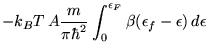
evaluating the derivative of the integrand at  ,
we get, to order ,
,
we get, to order ,
 |
(64) |
where  corresponds to the integral in Eq. (A15) and
 to the sum, and, from now on, we work per unit area.
The last term in Eq. (A16) is the change in
from
to the sum, and, from now on, we work per unit area.
The last term in Eq. (A16) is the change in
from  ,
the change in the chemical potential
due to the field, which is also of order .
,
the change in the chemical potential
due to the field, which is also of order .
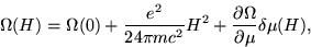
Substituting Eq. (A16) into in Eq. (A4) gives
 |
(65) |
where, from Eq. (A3), we have noted that
the contribution from cancels.
This cancellation occurs because
 , as noted in Eq. (A5).
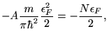
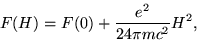
The magnetization is given by
 which
yields
which
yields
 with
with
 , the diamagnetic
susceptibility of free electrons per unit area in two dimensions, given by
, the diamagnetic
susceptibility of free electrons per unit area in two dimensions, given by
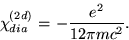 |
(66) |
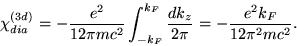
To get the corresponding result in 3- we need to add the motion in the
 -direction, specified by , and integrate from
  to
to  .
This is easy because Eq. (A18) is a constant independent of the
(2-) density of electrons (which would vary with ) and hence
the diamagnetic susceptibility of free electrons in 3- per unit volume
is given by
.
This is easy because Eq. (A18) is a constant independent of the
(2-) density of electrons (which would vary with ) and hence
the diamagnetic susceptibility of free electrons in 3- per unit volume
is given by
 |
(67) |
This is the expression first found by Landau. It is equivalent to Eqs. (31.72)
and (31.69) of Ashcroft and Mermin.
Next: About this document ...
Up: magnetic_field
Previous: Three dimensions and the
Peter Young
2002-10-31
![$\displaystyle -k_B T\, A{ m \over \pi \hbar^2}
\int_0^\infty \ln[ 1 + e^{\beta(\mu -
\epsilon)} ] \, d\epsilon$](img160.png)